
In my previous blog post I have explained the steps needed to solve a data analysis problem. Going further, I will be discussing in-detail each and every step of Data Analysis. In this post, we shall discuss about exploratory Analysis.
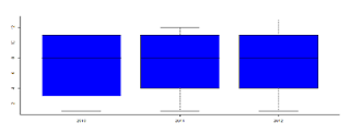
Box plot distribution of incidents occurring over the years.

What is Exploratory Analysis?
“Understanding data visually”
Exploratory Analysis means analyzing the datasets to summarize their main characteristics, often visually. This is the first step of any data analysis.
Objectives:
- Know the data types of the dataset – whether continuous/discreet/categorical
- Understand how the data is distributed
- Extract important input variables for the analysis
- Identify outliers
- To identity patterns, if exists
Exploratory Analysis Techniques:
- Box-Plot
- Histogram
- Trend analysis
- Scatter Plots
Let us understand the exploratory analysis by considering a data analysis problem.
Problem statement:
to analyze the incidents/events occurred over past 3 years and try to predict the event occurring in the future.
Solution:
After understanding the problem statement and gaining the sufficient domain knowledge, Identify the data sources & download the data into the programming environment.
The next step is to perform an Exploratory analysis as explained here. in today's post we shall look how exploratory analysis can be done.
Types of Exploratory analysis:
Type1: Understanding the data – variable names, dimensions of the dataset, data types of each and every variable.
data = read.csv("datasource.csv") #load data
dim(data) #know the dimensions of the data
[1] 839 50
Colnames(data) #know the column names
[1] "Incidents" "Year of Occurance" "Location.of.Occurrence" "Date.of.Occurence" [5]"Time.of.Occurrence" “Operational Phase”
Str(data) # know the data types of each of the variable – continuous/descrete/categorical
$ Incidents: int 41505 41537 41539 41565 41589 41596 41598
$ Vehicle.Type : Factor w/ 7 levels "","Volvo(all series)",..: 6 2 2 2 6 6
$ Location.of.Occurrence: Factor w/ 101 levels "","Abidjan","Accra",..: 53 35 35 35 96
$ Date.of.Occurence: Factor w/ 520 levels "1/1/2010","1/1/2012" ..: 1 32 37
Sum(!is.na(data$Date.of.Occurance) # counting the number of missing values in the column
Type2:Creating new varaibles/data type conversion suitable for the analysis – like factor variables into numerical,dates into year/month/day,time into hour of the day, etc. according to our convineince.
#Extracting year/month from Date of occurrence and creating new variables
xn = as.POSIXct(data$"Date.of.Occurence",format="%m/%d/%Y")
data["year"] = as.numeric(format(xn,"%Y"))
data["month"] = as.numeric(format(xn,"%m"))
str(data$"year")
num [1:839] 2010 2010 2010 2010 2010 2010
#extracting hour of the day and creating new variable TimeOfOccurance
(TOC)
data["TOC"] = sub(":.*", "", data$"Time.of.Occurrence")
str(data$"TOC")
chr [1:839] "18" "6" "21" "13" "16" "13" "11" "11" "15" "1" "13" "6"
Type3: Observe the summary of each and every variable to understand the variables.
summary(data$"Vehicle.Type")
Volvo (all series) ASHOK (all series) FIAT (all series) Maruthi (all series)
210 49 71 39
Type4: Decide which variables are good for analysis by using trends, boxplots, histograms etc.
boxplot(formula=as.numeric(data$"operational.Phase")~data$"year",col="blue")

Box plot distribution of incidents occurring over the years.
hist(data[which(data$"year" == 2011),]$"month",breaks = "Sturges",col=c('blue','red','green'),labels=T)

The above histogram depicts the month wise distribution of incidents occurred in 2011
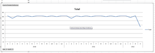
Trend analysis

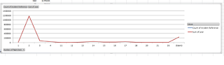
In the above graph, we can bring out the below inferences:
Sharp fall in the data in 2012 might be not capturing of the incidents
An average of 30 incidents occurring monthly
In the month of Feb there is sharp fall in the incidents

In the above trend image with graph in red color is plotted against Number of people in the deck and number of Incidents.
This clearly says that there is no relation between the Incident occurring and number of people in the deck.
Hope the above post gives you a very good understanding of how exploratory analysis can be done. In my next post we shall learn how to do forecasting using Linear regression.
MBA(Master of Business Administration) is a 2 year post graduate degree. This course covers different fields of such as marketing, accounting, logistics, management etc. Pursue your degree from BFIT. Admissions open for MBA in Dehradun.for more information visit our website:
ReplyDeletehttps://admission-kips-gncmh-kiits-kiims.bfitdoon.com/
You really make it seem so easy with your presentation but I find this topic to be really something that I think I would never understand. It seems too complex and extremely broad for me. I am looking forward for your next post, I will try to get the hang of it! industrial cleaning services
ReplyDeleteLooking for a reliable commercial plumber Houston? Our team specializes in providing top-quality plumbing services for businesses of all sizes. Whether it's new installations, routine maintenance, or emergency repairs, we've got you covered. With years of experience in the industry, we handle everything from drain cleaning and leak detection to complex pipe installations.
ReplyDeleteWe pride ourselves on delivering fast, efficient service with minimal disruption to your operations. Fully licensed, insured, and available 24/7, we ensure your plumbing systems are always in excellent condition. Trust us for professional, affordable plumbing solutions in Houston. Contact us today for a free consultation and estimate!
This was a lovely blog posst
ReplyDelete